Code Design
This section of the documentation describes the data structures and organisation of the code for InDiCA. It is primarily intended for developers.
Data Containers
Diagnostics and the results of calculations are stored using the
xarray.DataArray and xarray.Dataset
classes. This stores multidimensional data with labelled dimensions,
coordinates along each dimension, and associated metadata. Standard
mathematical operations are built into these objects. Additional
bespoke functionality is provided using meta-data and “custom
accessors”,
as described in the xarray documentation.
Each observed quantity will be stored in its own
xarray.DataArray object. Results describing the same
species of in the plasma can be grouped together by the user into a
single xarray.Dataset. This will allow the data to be
passed to a calculation as one argument, rather than several and it is
anticipated that most calculations will be designed to work this way.
Metadata
The following metadata should be attached to
xarray.DataArray objects:
- datatype
(str, str) Information on the type of data stored in this
xarray.DataArrayobject. See Data Value Type System.- provenance
prov.model.ProvEntity Information on the process which generated this data, including the equilibrium used, if set. See Provenance Tracking.
- partial_provenance
prov.model.ProvEntity Information on the process which generated this data, not including the equilibrium used. See Provenance Tracking.
- transform
indica.converters.CoordinateTransform An object describing the coordinate system of this data, with methods to map to other coordinate systems. See Coordinate Systems and Transforms
- error (optional)
xarray.DataArray Uncertainty in the value (will not contain any metadata of its own).
- dropped (optional)
xarray.DataArray Any channels which were dropped from the main data.
In addition, where xarray.Dataset objects are used, they
will have the following metadata:
- provenance
prov.model.ProvEntity A provenance
collectionindicating the contents of this Dataset. See Data Value Type System.- datatype
(str, dict) Information on the type of data stored in this
xarray.Datasetobject. See Data Value Type System.
Accessing Equilibrium Data
Key to analysing any fusion reactor data is knowing the equilibrium state of the plasma. This is done using equilibrium calculations. Multiple models are available for this and it should be easy to swap one for another in the calculation. The same interface should be used for results from all fusion reactors (as is the case elsewhere in the code).
The equilibrium data which is of interest is the total magnetic field
strength, the location of various flux surface (poloidal, toroidal,
and potentially others), the minor radius, the volume enclosed by a
given flux surface, and the minimum flux surface for a line-of-sight
(impact parameter). An Equilibrium
class is defined with methods to obtain these values. Rather than try
to anticipate every type of flux surface which might be needed, any
method which takes or returns a flux surface has an argument kind
which accepts a string specifying which one is desired
("poloidal", by default). There is also a method to convert
between different flux surface types. This will allow support to be
added for additional kinds of fluxes without needing to change the
interface.
Unfortunately, equilibrium results are not always entirely accurate
and may need to be adjusted. The location of the flux surfaces will often be
slightly offset along the major axis from the “real” ones. Therefore,
the user can pass in R_shift and z_shift arguments to the
constructor, indicating how much the flux surfaces should be moved by
in each direction. It is also possible to pass an a DataArray
containing electron temperatures. If this is present, then instead of
using the specified R_shift the constructor will attempt to
determine an optimal one. It estimates (to the nearest
half centimetre) the offset in R needed for the electron temperature
at the last closed flux surface to be about 100eV. It provides a plot
of the optimal R-shift at different times, with the average value also
draw. This average value is used to reposition the flux surfaces and a
second plot is produced with electron temperature against normalised
flux. The user can choose to accept this offset or to specify a custom
value. If the latter, these plots will be recreated with the new
R-shift and the user will again be asked whether or not to accept
it. (This is the default behaviour; it is also possible for the user
to provide a handler function with custom functionality, such as
determining the result automatically or to integrate the selection
interface more tightly with the GUI.)
Equilibrium objects are instantiated using a
dictionary of xarray.DataArray objects obtained using a
DataReader object (see Data IO). The equilibrium
class can be represented by the following UML.
![class Equilibrium {
+ tstart: float
+ tend: float
+ provenance: ProvEntity
- _session: Session
+ __init__(equilibrium_data: Dict[str, DataArray], T_e: DataArray,
\t\t\tR_shift: float, z_shift: float)
+ Btot(R: DataArray, z: DataArray, t: DataArray): (DataArray, DataArray)
+ enclosed_volume(rho: DataArray, t: DataArray, kind: str):
\t\t\t\t\t\t\t(DataArray, DataArray)
+ invert_enclosed_volume(vol: DataArray, t: DataArray, kind: str):
\t\t\t\t\t\t\t(DataArray, DataArray)
+ minor_radius(rho: DataArray, theta: DataArray, t: DataArray,
\t\t\tkind: str): (DataArray, DataArray)
+ flux_coords(R: DataArray, z: DataArray, t: DataArray, kind: str):
\t\t\t\t\t\t\t(DataArray, DataArray, DataArray)
+ spatial_coords(rho: DataArray, theta: DataArray, t: DataArray,
\t\t\tkind: str): (DataArray, DataArray, DataArray)
+ convert_flux_coords(rho: DataArray, t: DataArray, from_kind: str,
\t\t\tto_kind: str): (DataArray, DataArray)
+ R_hfs(rho: DataArray, t: DataArray, kind: str): (DataArray, DataArray)
+ R_lfs(rho: DataArray, t: DataArray, kind: str): (DataArray, DataArray)
}](_images/plantuml-b78db9fee23efb38136ea6106e03944650e1447d.png)
Coordinate Systems and Transforms
Each diagnostic which is used for calculations is stored on a different coordinate system and/or grid. One of the key challenges is thus to make it easy to convert between these coordinate systems. This is further complicated by the fact that many of the coordinate systems are based on what (time-dependent) equilibrium state was calculated for the plasma. Transforms between coordinate systems must therefore be agnostic as to which equilibrium results are used.
When operations are performed on xarray.DataArray objects,
they are automatically aligned
(“alignment” meaning that ticks on their respective axes have the same
locations). Any indices which do not match are discarded; the result
consists only of the intersection of the two sets of coordinates. When
operating on datasets where some or all dimensions have different
names, it automatically performs Broadcasting by dimension name. However,
note that this would not be physically correct if the coordinates are
not linearly independent.
There is also built-in support for interpolating onto a new coordinate system. This can be either for different grid-spacing on the same axes or for another set of axes entirely. Unfortunately, only 1st order interpolation is supported if interpolating over multiple dimensions. This is all a bit cumbersome, so convenience methods are provided to make it easier.
In order to perform these sorts of conversions, a means is necessary to map from one coordinate system to another. An arbitrary number of potential coordinate systems could be used and being able to map between each of them would require \(O(n^2)\) different functions. This can be reduced to \(O(n)\) if instead we choose a go-between coordinate system to which all the others can be converted. A sensible choice for this would be \(R, z\), as these axes are orthogonal, the coordinates remain constant over time, and libraries to retrieve equilibrium data typically work in these coordinates.
A CoordinateTransform class is defined to handle
this process. This is an abstract class which will have a different
subclass for each type of coordinate system. It has two abstract
methods, for converting coordinates to and from
R-z. A non-abstract convert_to method takes
another coordinate system as an argument and will map coordinates
onto it. Finally, the distance method can provide the spatial
distance between grid-points along a given axis and first grid-point
on that axis.
Note
If you wish to convert the coordinates used by a particular
xarray.DataArray into a different coordinate system, do
not call transform’s methods directly. Instead you should use
convert_coords() or
get_coords(). The
only difference between the two is the latter will also return the
time coordinates. These methods are simpler and will also cache
results to save needing to recalculate them if they are needed
again later.
In addition to doing conversions via R-z coordinates, subclasses of
CoordinateTransform may define
additional methods to map directly between coordinate systems. This
would be useful if there is a more efficient way to do the conversion
without going through R-z, if that transformation is expected to be
particularly frequently used, or if that transformation would need to
be done as a step in converting to R-z coordinates. These can be
accessed by calling
get_converter() with
the coordinate transform that you wish to convert to. If a shortcut
method is available for this conversion, it will be
returned. Otherwise, None will be returned. It is the responsibility
of the writer of the subclass to override this method, if necessary.
Each subclass should indicate the names of the two spatial dimensions associated with the coordinate system. In some cases these can be specified as static attributes (when the coordinate is universal, such as R, z, and rho_poloidal) while in others they should be object attributes (e.g., when it corresponds to channel numbers for a particular instrument).
The CoordinateTransform class is agnostic
to the equilibrium data and can be instantiated without any knowledge
of it. However, many subclasses will require equilibrium information
to perform the needed calculations. This can be set using the
set_equilibrium() method
at any time after instantiation. Calling this method multiple times
with the same equilibrium object will have no affect. Calling with a
different equilibrium object will cause an error unless specifying the
argument force=True.
![abstract class CoordinateTransform {
+ x1_name: str
+ x2_name: str
+ set_equilibrium(equilibrium: Equilibrium, force: bool)
+ get_converter(other: CoordinateTransform, reverse: bool): Optional[Callable]
+ convert_to(other: CoordinateTransform, x1: DataArray, x2: DataArray,
\t\tt: DataArray): (DataArray, DataArray, DataArray)
+ {abstract} convert_to_Rz(x1: DataArray, x2: DataArray, t: DataArray):
\t\t\t\t\t\t(DataArray, DataArray, DataArray)
+ {abstract} convert_from_Rz(x1: DataArray, x2: DataArray, t: DataArray):
\t\t\t\t\t\t(DataArray, DataArray, DataArray)
+ distance(direction: int, x1: DataArray, x2: DataArray,
\t\tt: DataArray): (DataArray, DataArray)
- encode(): str
- {static} decode(input: str): CoordinateTransform
}](_images/plantuml-3041b35737df06110ec4f903d08461ab0d5a608a.png)
Methods to encode() and
decode() a transform
to/from JSON will be provided. This will work by encoding the
arguments used to instantiate a transform object, allowing it to be
recreated upon decoding. Note that this means the equilibrium will
still need to be set again manually. Most of this functionality should
be implemented from the base class and those writing subclasses
shouldn’t need to do more than call a method at instantiation or use a
decorator (details TBC).
Each DataArray will have a transform attribute which is one of
these objects. To save on memory and computation, different data from the same
instrument/diagnostic will share a single transform object. This
should not normally be of any concern for the user, unless they are
attempting to use multiple sets of equilibrium data at once.
The methods on CoordinateTransform take
xarray.DataArray objects as arguments. They make use of
broadcasting by dimension name. This
allows easy creation of grids.
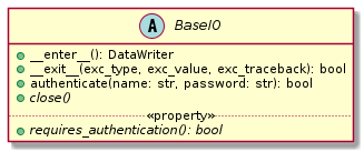
Data IO
There is some common functionality for all reading and writing
operations which will be performed. This involves authenticating
users and opening/closing the IO stream. For convenience, methods
should be provided to make the latter possible through a context
manager. This functionality is placed in a common base class
BaseIO, leaving methods abstract where
necessary.
Input
Diagnostics
Reading data is done using a standard interface,
DataReader. A different subclass is
defined for each data source/format. These return collections of
xarray.DataArray objects with all the necessary metadata.
![abstract class DataReader {
+ {static} NAMESPACE: (str, str)
- {static} _AVAILABLE_QUANTITIES: dict
+ {abstract} INSTRUMENT_METHODS: dict
- {abstract} _IMPLEMENTATION_QUANTITIES: dict
__
+ get(uid: str, instrument: str, revision: int,
\t\t\t\tquantities: Set[str]): Dict[str, DataArray]
+ get_thomson_scattering(uid: str, instrument: str, revision: int,
\t\t\t\tquantities: Set[str]): Dict[str, DataArray]
- {abstract} _get_thomson_scattering(uid: str, instrument: str, revision: int,
\t\t\t\tquantities: Set[str]): Dict[str, Any]
+ get_charge_exchange(uid: str, instrument: str, revision: int,
\t\t\t\tquantities: Set[str]): Dict[str, DataArray]
- {abstract} _get_thomson_scattering(uid: str, instrument: str, revision: int,
\t\t\t\tquantities: Set[str]): Dict[str, Any]
etc.
+ available_quantities(instrument: str): Dict[str, (str, str)]
}
class PPFReader {
+ NAMESPACE: (str, str)
+ {static} INSTRUMENT_METHODS
- {static} _IMPLEMENTATION_QUANTITIES: dict
- _client: SALClient
__
+ __init__(pulse: int, tstart: float, tend: float, server: str)
+ authenticate(name: str, password: str): bool
- _get_thomson_scattering(uid: str, instrument: str, revision: int,
\t\t\t\tquantities: Set[str]): Dict[str, Any]
- _get_thomson_scattering(uid: str, instrument: str, revision: int,
\t\t\t\tquantities: Set[str]): Dict[str, Any]
etc.
+ close()
.. «property» ..
+ {abstract} requires_authentication(): bool
}
abstract class BaseIO
BaseIO <|-- DataReader
DataReader <|-- PPFReader](_images/plantuml-fbee8af71d9b314020d07120e62ae4787c4959e9.png)
Here we see that reader classes contain public methods for getting
data for each type of diagnostic. It also provides methods for
authentication and closing a database connection. Each reader should
feature a dictionary called _IMPLEMENTATION_QUANTITIES. This is a
dictionary which maps from instrument names to more dictionaries. This
second layer of dictionaries maps from the names of available
quantities for that instrument to the data type of each one. Subclasses should also provide a dictionary
called INSTRUMENT_METHODS which maps from instrument names to the
particular method needed to retrieve the data for that
instrument. This is needed for the general
get() method to work. Finally, the
NAMESPACE attribute can be overridden for use in PROV data. The first element of the tuple should be a
short name for the namespace, while the second should be a URL
associated with the data (e.g., the URL of the server from which is
fetched).
The methods for getting diagnostic data (e.g.,
get_thomson_scattering()) method is
implemented in the parent class and provides basic functionality for
assembling raw NumPy arrays into xarray.DataArray objects,
with appropriate metadata. The actual process of getting these arrays
data is delegated to the abstract private methods (in this case,
_get_thomson_scattering), which are implementation
dependent. Implementations are free to define additional private
methods if necessary. The form of the constructor for each reader
class is not defined, as this is likely to vary widely.
Lines of Sight
Note that the PPF reader must read data on line of sight positions
from a separate datafile, referred to as SURF. This is done using
read_surf_los(). Currently the PPF
reader is hardcoded to call this for a version of the SURF database
file distributed with InDiCA. However, in future it may be extended to
allow users to specify an alternate version.
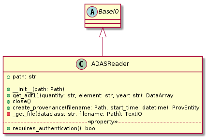
Atomic Data
In addition to reading in diagnostics, it is necessary to load ADAS
atomic data. Fortunately, this is much more straightforward. A simple
ADASReader class is defined with method
for getting different types of atomic data. Currently only ADF11 data
is supported, via the get_adf11()
method. By default, data is fetched from the OpenADAS database and then cached on the disk for
reuse. Alternatively, at construction, the user may provide a path to
a file hierarchy containing proprietary ADAS data. The get...
methods returns a xarray.DataArray objects, with
properties (e.g., temperature, density, charge state) used as
coordinates.
Output
Warning
Data output is not yet implemented and may undergo changes once it has been.
A similar approach of defining an abstract base class
(indica.writers.DataWriter) is used for writing out data to
different formats.
![abstract class DataWriter {
+ write(uid: str, name: str, *args: Union[DataArray, Dataset])
- {abstract} _write(uid: str, name: str, data: Dataset, equilibria: Dict[str, Equilibrium], prov: ProvDocument)
}
class NetCDFWriter {
+ __init__(filename: str)
+ _write(uid: str, name: str, data: Dataset, equilibria: Dict[str, Equilibrium], prov: ProvDocument)
+ close()
.. «property» ..
+ requires_authentication(): bool
}
abstract class BaseIO
BaseIO <|-- DataWriter
DataWriter <|-- NetCDFWriter](_images/plantuml-158b71463d1eb07339201256800cb6272c214180.png)
In derived class in this example writes to NetCDF files, which is a particularly easy task as there is already close integration between xarray and NetCDF. Other derived classes will be defined for each database system which the software is able to read from.
This is a simpler design than that used for reading data. This is
because reading data requires dealing with the particularities of how
each diagnostic is stored data in the database and reorganising that
into a consistent format. When writing we can rely all diagnostics
being represented in essentially the same way in memory and thus only
need to convert it into a writeable format once, in the
indica.writers.DataWriter.write() method. The only task
remaining is the simple one of writing to disk or a database in the
private _write method.
To reformat data to be more amenable to writing, the following will
occur. All data will be placed in a new xarray.Dataset
containing all data, with attributes reformated as necessary:
Uncertainty will be made a member of the dataset, with the name
VARIABLE_uncertainty, whereVARIABLEis the name of the variable it is associated with.Dropped data will be merged into the main data and the attribute will be replaced with a list of the indices of the dropped channels and
dropped_dim, the name of the dimension these indices are for.The coordinate transform will be replaced with a JSON serialisation, from which it can be recreated. These serialisations will be stored in a dictionary attribute for the Dataset as a whole, with each DataArray holding the key for its corresponding transform.
The PROV attributes will be replaced by the ID for that entity. The complete PROV data for the session will be passed to low-level writing routines as a separate argument.
Datatypes will be serialised as JSON
All variables will have an
equilibriumattribute, which provides an identifier for the equilibrium data (passed to the low-level writer in a dictionary).
PROV and equilibrium data should be written elsewhere in the output file/database, with attributes used to associate variables with it. If desired, a similar approach could be taken when it comes to writing coordinate transform data, as many variables are likely to share the same transform.
Data Value Type System
When performing physics operations, arguments have specific physical meanings associated with them. The most obvious way this manifests itself is in terms of what units are associated with a number. However, you may have multiple distinct quantities with the same units and an operation may require a specific one of those. It is desirable to be able to detect mistakes arising from using the wrong quantity as quickly as possible. For this reason, operations on data define what they expect that data to be and to check this.
Beyond catching errors when using this software as a library or interactively at the command line, this technique will be valuable when building a GUI interface. It will allow the GUI to limit the choice of input for each operation to those variables which are valid. This will simplify use and make it safer.
This system does not need to be very complicated. A type for the data
in an xarray.DataArray consists of two labels. The first
indicates the general type of quantity (e.g., number density,
temperature, luminosity, etc.) and the second indicates the specific
type of species (type of ion, electrons, soft X-rays, etc.) which
this quantity describes. These are combined in a
2-tuple. Either element of the tuple may also be None, indicating
that the type is unconstrained or unknown. See examples below:
# Describes a generic number density of some particle
("number_density", None)
# Describes number density of electrons
("number_density", "electrons")
# Describes number density of primary impurity
("number_density", "tungsten")
Type descriptions are a bit more complicated for
xarray.Dataset objects. Recall that these objects are
groupings of data for a given species. Therefore, they are made up a
2-tuple where the first item is the specific type and the second is a
dictionary. This dictionary maps the names of the
xarray.DataArray objects contained in the Dataset to the
general type that DataArray stores:
# Describes data number density, temperature, and angular
# frequency of Tungsten
("tungsten", {"n", "number_density",
              "T": "temperature",
              "omega": "angular_freq"})
Each operation on data contains information on the types of arguments
it expects to receive and return and has a method to confirm that
these expectations are met. An operation may leave the
general and/oror specific datatype as None. Each
xarray.DataArray and xarray.Dataset contains
type information in its metadata, associated to the key "datatype" and
this always specifies both general and specific type(s).
In principal, this is all the infrastructure that would be needed for the type system. However, it is useful to keep a global registry of the types available. This helps to enforce consistent labelling of types and gives the ability to check for type. It is also used to store information on what each type corresponds to and in what units it should be provided. This information is useful documentation for users and can be integrated in a GUI interface. This is be accomplished using dictionaries:
GENERAL_DATATYPES = {"number_density": ("Number density of a particle", "m^-3"),
                     "temperature": ("Temperature of a species", "keV")}
SPECIFIC_DATATYPES = {"electrons": "Electron gas in plasma",
                      "tungsten": "Tungsten ions in plasma"}
This information is stored in the datatypes module.
It is expected that many calculations will not specify a specific datatype as they can in principle work with any kind of ion. The user can try running the calculation with different combinations of impurities and see which produces the most reasonable results.
Provenance Tracking
In order to make research reproducible, it is valuable to know exactly how a data set is generated. For this reason, the library contains a mechanism for tracking data “provenance”. Every time data is created, either by being read in or by a calculation on other data, a record should also be created describing how this was done.
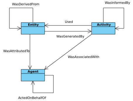
There already exist standards and library for recording this sort of information: W3C defines the PROV standard and the PyProv library exists to use it from within Python. In this model, there are the following types of records:
- Entity
prov.model.ProvEntity Something you want to describe the provenance of, such as book, piece of artwork, scientific paper, web page, or book.
- Activity
prov.model.ProvActivity Something occurring over a period of time which acts on or with entities.
- Agent
prov.model.ProvAgent Something bearing responsibility for an activity occurring or an entity existing.
There are various sorts of relationships between these objects, with the main ones summarised in the diagram below.
This software provides a class Session which holds
the provenance document as well
as contains information about the user and version of the software. A
global session can be established using
indica.session.Session.begin() or a context manager. Doing so
requires specifying information about the user, such as an email or
ORCiD ID. The library will then use this global session to record
information or, alternatively, you can provide your own instance when
constructing objects. The latter option allows greater flexibility
and, e.g., running two sessions in parallel.
What follows is a list of the sorts of PROV objects which will be generated. Each of them should come with an unique identifier. Where the data is read from some sort of database this could be the key for the object. Otherwise it should be a hash generated from the metadata of the object.
Calculations
A calculation will be represented by an Activity. It will be linked with the data entities it used to do the calculation, the user or other agent to invoke it, and the Operator object which actually performed it.
xarray.DataArray objects
Each data object will be represented by an Entity. This entity will
contain links with the user and piece of software (e.g., reader or
operator) to create it, the reading or calculation activity it was
produced by, and any entities which went into its creation. This first
entity will be stored as an attribute with the key
partial_provenance.
An additional Entity (a collection)
will be stored as an attribute with key provenance. This
collection will contain the partial_provenance entity and the
entity for the indica.equilibrium.Equilibrium object used by
this data. Any change to the equilibrium object will result in a new
provenance entity.
xarray.Dataset objects
Datasets will also be represented by Entities, specifically a collection. The DataArray objects making up the dataset will be indicated in PROV as members of the collection.
DataReader objects
These objects are represented as both an Entity and an Agent. The former is used to describe how it was instantiated (e.g., the user that created it, what arguments were used) while the latter can be used to indicate when it creates DataArray objects by reading them in.
Dependency
Third-party libraries which are depended on should be represented as Entitites in the provenance data. Information should be provided on which version was used.
Equilibrium objects
An Equilibrium object will be represented by an Entity. This references the user (agent) to instantiate it, the constructor call (activity) that did so, and the data (entities) used in its creation.
External data
External data (e.g., contained in files or remote databases) should have a simple representation as an Entity. Sufficient information should be provided to uniquely identify the record.
Operator objects
Similar to reader objects, these are represented as both an Entity and an Agent. Again, the former provides information on who created the operator and what arguments were used. The latter indicates the object’s role in performing calculations.
Package
The overall library/impurities package is itself represented by an Entity. This should contain information on the version or git commit. It could also provide information on the authors who wrote it.
Reading data
Reading data is an Activity. It is associated with a reader agent and a user of the software. It uses external data entities.
Session objects
An Activity representing the current running instance of this software. It uses the package and dependencies and is associated with the user to launch it. It contains metadata on the computer being used, the working directory, etc.
Users
The person using the software is represented as an Agent. Data objects will be attributed to them. They are associated with the session. Sometimes they will delegate authority to classes or functions which are themselves agents. Sufficient metadata should be provided to allow them to be contacted. Ideally they would have some sort of unique identifier such as an ORCiD ID, but email is also acceptable.
xarray Extensions
A number of InDiCA-specific utilities are needed in addition to
standard xarray functionality. For this reason, “custom accessors”
were written to provide these methods in the indica
namespace. Accessors are available for both
xarray.DataArray and xarray.Dataset objects,
although the functionality varies between them. These accessors are
available in any scope that has imported the top-level indica
package.
If you want to convert the coordinates used by a given DataArray into
a coordinate system given by new_transform, this
can be done by calling
convert_coords()
or get_coords().
# Get new spatial coordinates
x1, x2 = array.indica.convert_coords(new_transform)
# Or, to get t as well:
x1, x2, t = array.indica.get_coords(new_transform)
To interpolate data onto the coordinate system used by another
DataArray, use the
get_coords() method. This
allows you to do maths with DataArrays using different coordinate
systems:
# array1 and array2 are on different coordinate systems.

# Broadcasting creates a 4D array; probably not what you want
array3 = array1 + array2

# Same coordinate system as array1
array4 = array1 + array2.indica.remap_like(array1)

# Same coordinate system as array2
array5 = array1.indica.remap_like(array2) + array2
Other functionality provided by the DataArray accessor includes
Indicating data which should be dropped/ignored
Restoring dropped data
Getting/setting the equilibrium object
Checking datatype
Performing cubic 2D interpolation
For Datasets you can
convert coordinates (if metadata contains key
"transform")add new data, updating provenance accordingly
Get the datatype and check others are compatible
Read the full documentation for data for more details.
Operations on Data
In the previous sections I referred to “operations” on data. These
should be seen as something distinct from standard mathematical
operators, etc. Rather, they should be thought of as representing some
discreet, physically meaningful calculation which one wishes to
perform on some data. They take physical quantities as arguments and
return one or more derived physical quantities as a result. They are
represented by callable objects of class
indica.operators.Operator. A base class is provided,
containing some utility methods, which all operators inherit from. The
main purpose of these utility methods is to check that types of
arguments are correct and to assemble information on data
provenance. The class is represented by the following UML:
![class Operator {
- _start_time: datetime
- _input_provenance: list
- _session: Session
+ agent: ProvAgent
+ entity: ProvEntity
+ {abstract} ARGUMENT_TYPES: list
+ __init__(self, sess: Session, **kwargs: Any)
+ {abstract} return_types(self, *args: DataType): tuple
+ {abstract} __call__(self, *args: Union[DataArray, Dataset]): Union[DataArray, Dataset]
+ assign_provenance(data: Union[DataArray, Dataset])
+ validate_arguments(*args: Union[DataArray, Dataset])
+ {static} recreate(provenance: ProvEntity): Operator
}
class ImplementedOperator {
+ ARGUMENT_TYPES: list
+ RESULT_TYPES: list
+ __init__(self, ...)
+ __call__(self, ...): Union[DataArray, Dataset]
}
Operator <|-- ImplementedOperator](_images/plantuml-84d34077b04eaa25d2bbda17db5a934f112b8c39.png)
Each operator object should have an attribute called ARGUMENT_TYPES,
which may be either a class or an object attribute, as
appropriate. This is a list of datatypes. Specific and/or general
datatypes may be left as None, if they are not constrained. The
last element in the list may be ellipsis dots. This indicates that
operator is variadic. The types of the variadic argument must match
the penultimate item in INPUT_TYPES (i.e., the one preceding the
ellipsis). If that item contains a None field, then the datatype
of the corresponding argument must also be matched. For example:
assert operator.ARGUMENT_TYPES == [("luminous_flux", None), ...]
assert sxr_h.attrs["datatype"] == ("luminous_flux", "sxr")
assert sxr_v.attrs["datatype"] == ("luminous_flux", "sxr")
assert bolo_h.attrs["datatype"] == ("luminous_flux", "bolometric")
# This would be a valid call
operator(sxr_h, sxr_v)
# This would not be valid
operator(sxr_h, bolo_h)
There is also an abstract method
return_types().
This takes datatypes as arguments, corresponding to the positional
arguments with which the operator would be called. It returns a tuple
of the datatypes which it would produce.
While performing the calculation they should not make reference to any global data except for well-established physical constants, for reasons of reproducibility and data provenance. If it would be too cumbersome to pass all of the required data when calling the operation, additional parameters can be provided at instantiation-time; this is useful if the operation is expected to be applied multiple times to different data but using some of the same parameters.